This section discusses image processing generically, assuming you will be able to apply its concepts with the software package of your choice. Excellent image processing programs for the amateur include AIP4WIN, MaxIm DL, MIRA, MegaFix, IRIS, PixInsight, and AstroArt. I use AIP4WIN and PhotoShop, primarily, with an occasional application from PixInsight. All pictorial processing examples in this document were done with AIP4WIN.
a. Calibrating With Master Darks. The first step in processing a light frame is to subtract a matching, high-SNR master dark frame. The purpose of this is to remove the thermal signal which was built up in the light integration. The master dark is made to match the light frame either by making the light and dark integrations the same exposure times or by scaling down longer dark integrations. Scaling up shorter dark integrations does not work.
An added complication to dark scaling is the requirement of subtracting a master bias frame from both the light frame and the master dark before scaling and subtracting the master dark. This is necessary because the buildup of time-dependent thermal signal cannot be properly scaled unless the baseline value of the bias signal is removed. A good master bias frame can be made by averaging five dark frames of the shortest possible integration time (0.1 second or less).
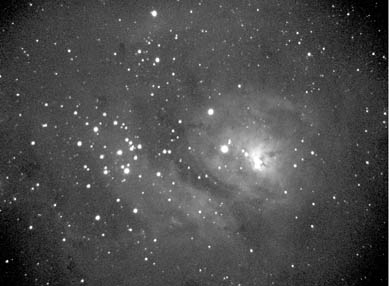
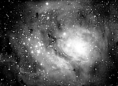
Here is a "before" and "after" example of dark calibration:
Raw 4-minute integration of the
Lagoon nebula (stretched)
Matching 4-minute dark frame
(stretched) 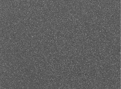
Raw image after dark subtraction
(stretched) 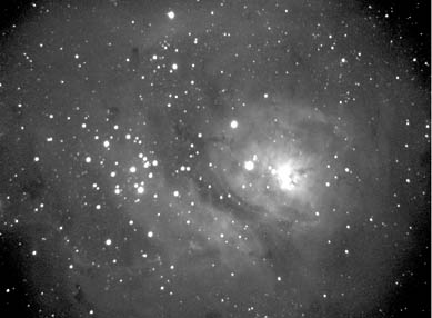
b. Calibrating With Master Flats. The second step in image calibration is to "flatten" the light frame with a high-SNR master flat-field frame. This calibration step can be ignored for "pretty picture" purposes if the sky background does not look uneven or appear to be distorted by artifacts (such as the halo-shaped shadows of dust specks on the optical surfaces near the chip); however, if the image will be used for scientific data or has a noticeably uneven background due to vignetting or replicable optical blockages and reflections, then flat-fielding is called for. The arithmetic application of flat fielding is often referred to as simple division, but what actually happens is that the value of each pixel in the flat is divided by the mean pixel value, then each result is divided into the corresponding pixel value in the light frame.
Flats are different than light frames in many ways, but the important difference for the purposes of this discussion is that the field of view (FOV) of a flat has no frame of reference against celestial objects (this is true even for sky flats). Unlike flat frames, there frequently is sky movement between object frames and that is often good, since some processing algorithms work better when there has been a little offset among stacked frames. Flats, on the other hand, are intended to be stacked on top of each other, pixel position by pixel position in each frame array (i.e., 1,1 stacks on 1,1; 5,5 on 5,5; 115,236 on 115,236; etc.). Thus, stacking and averaging uncalibrated (i.e., non-dark-subtracted) flats result in a higher-SNR uncalibrated flat. This is the same as stacking/averaging numerous dark frames to achieve a higher-SNR master dark. The easiest way to make a good master flat is, therefore, to average several uncalibrated flats and then calibrate the result with a master dark frame....two averaging sequences then one calibration step.
Light frames are different. They are intended to stack the sky objects...usually stars...on top of themselves to improve the SNR of the desired images, thus the same pixel position in each frame is almost invariably shifted slightly for each frame that makes up the stack. For the pixels to be properly calibrated, each frame must be calibrated with a master dark (and flat, if needed) before stacking.
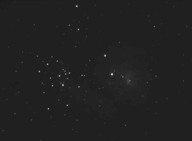
Here is the master flat that was made through the same telecompressed C8 optical system as the Lagoon images:
Flat-field frame (stretched) 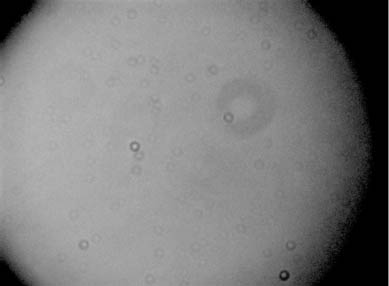
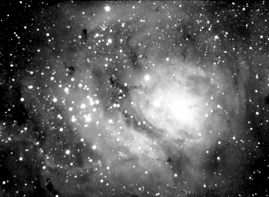
Here is the above image of the dark-calibrated Lagoon Nebula after flat-field calibration:
Lagoon image after flat-field
calibration (stretched) 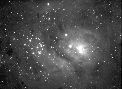
c. Scaling and Stacking Subexposures. Calibrated images can be stacked to improve the SNR. Stacking five well-calibrated 4-minute integrations can create the equivalent of one well-calibrated 20-minute integration. Good image-processing programs will allow the user to set up an automatic sequence of image calibration and stacking for any number of subexposures. Good programs will also provide a 2-star image rotation and registration algorithm that will automatically stack images which have field rotation and shifting among the frames. If there has been field rotation during image acquisition with a camera having non-square pixels, the images should be resampled to square the pixels before stacking is attempted.
Subexposures should be reviewed either before or during stacking to determine if they should be retained in the stack. Programs such as AIP4WIN, which comes on a CD-ROM with the “Handbook of Astronomical Image Processing” from Willmann-Bell ( http://www.willbell.com ), allow manual review of each subexposure as it is stacked. If the calibrated image is very poor compared to its brethren, due to tracking errors, incident light, or major artifacts, such as a bright airplane or satellite trail, then it should not be retained. Experience is the best teacher when it comes to retention decisions.
The three basic options for stacking methodology are summing, average combining, and median combining. Summing and averaging provide the best SNR results and are essentially the same mathematical algorithm if 32-bit floating point arithmetic is used by the program and the program scales the sum back into the 16-bit display range. If summing is not done this way by a program and it would result in saturation of many pixels in the summed image, then averaging is the better alternative. When averaging images, it is good to select a prescaling factor (a simple pixel value multiplier) to apply to each calibrated image before stacking, especially if the subexposures are short and the object of interest shows very low pixel values in each subexposure. You should select a multiplier which does not push pixel values to saturation levels, but which will deliver significantly more grayscale values to the stacked average. Without prescaling, very “underexposed” images may show visible, undesirable grayscale gradations in the final stack. Median combining is useful for stacking three or more images with variable artifacts in each image. A median combination will assign the middle value in the stack to each pixel, thus obviating the effects of extra high or low values. This is primarily useful for combining numerous dark frames, automatically eliminating the unwanted effects of cosmic ray hits in the images. You should be aware, though, that median combining results in lower SNR than averaging (NOTE: some programs are implementing a "Sigma" combine that retains good SNR while ignoring unusual pixel values, such as cosmic-ray hits)
When using scaling multipliers in stacking filtered images, such as RGBs, make sure and use the same multiplier for each color set, otherwise the color balancing factors to be applied later will be thrown off. This caveat applies whether the filtered subexposures had the same integration times or not. For example, if you have determined (more on this later) that your system is only 50% as sensitive to blue as it is green and red, then you may choose to either shoot all filtered subexposures at the same integration time (and just take 50% more blues for SNR purposes) or shoot the same number of blues but each at a 50% longer integration time. I prefer to make all integrations the same length; but, either way, any scaling multiplier used during stacking should be constant for all three stacks.
Here is the image of the Lagoon Nebula after calibrating and stacking four 4-minute integrations:
Stack of four Lagoon images
(stretched) 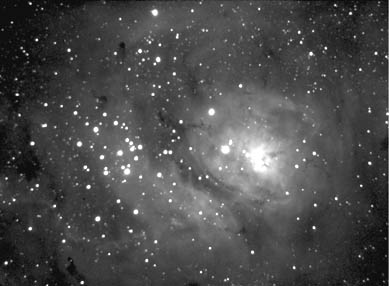
d. Processing a Luminance Image (monochrome image processing). Once the stacking is done, the next step should be to process the unfiltered image using mathematical transfer functions, mathematical filters, and other algorithms. The object here is to process the image data so that it is displayed across the full 16-bit range of the standard FITS file format in a way that shows the object(s) of interest most effectively and esthetically.
Before stretching or filtering the file data, unacceptable artifacts, such as large blooming spikes and hot pixels resulting from cosmic ray hits, should be removed. Most programs have pixel editing functions which can be used on individual pixels or pixel areas to eliminate the artifacts. Care should be taken not to create data or to remove true astronomy data, but removal of blooming spikes cannot help but “blank out” areas where the spikes exist. Such editing may or may not be better than just leaving the spikes in the image, but some programs have very effective functions dedicated specifically to the esthetic removal of blooming spikes. If there are a number of individual hot pixels scattered randomly in the image, a noise filtering function using a numerical median mask may offer the best solution. Look for a “noise filter”in your program menu.
As a final step before image stretching and filtering, the image aspect ratio should be resampled if the native CCD pixels are not square. For example, if the pixels are 15 microns wide by 12 microns tall and the array is 500 pixels wide (500 columns) by 500 pixels tall (500 rows), then the array should be resampled to 625 pixels wide by 500 pixels tall so that the square pixels on output devices will show the sky dimensions correctly.
Sometimes an unavoidable and uncalibratible background gradient appears in an image due to local light scatter during acquisition. These should be dealt with next. Some programs have gradient removal tools which are very effective in dealing with these. The easiest gradients to fix are those with a slow, linear change in one direction across the image. These can usually be “flattened” by introducing an opposite gradient to the pixel values in the array. The toughest gradients (other than vignetting, which should be dealt with by flat-fielding), are circular ones which are basically hot spots resulting from internal optical reflections. These require special gradient removal tools, such as those in AIP4WIN.
A deconvolution is a filtering process that uses Fourier transform mathematics to improve the resolution or sharpness of an image. This process uses a sample of the image point spread function (PSF), as represented by an unsaturated star, or a theoretical PSF, as represented by a Gaussian profile, to modify the image as if its PSF were much smaller and more uniform. This is the type of filter that was used to successfully improve the Hubble Space Telescope images until its optics were repaired. Images that have good pixel sampling of the PSF and have high SNR are good candidates for deconvolutions. Deconvolutions run on lesser images usually produce unacceptable artifacts, such as dark haloes or blotches around stars and blotchy sky backgrounds. If an image looks like a good candidate for deconvolution, it normally should be performed before any other filters or stretches are applied. There are several types of deconvolution algorithms, including Richardson-Lucy (RL), Van Cittert, and Maximum Entropy (MED). For deep-sky images, I much prefer the RL algorithms, especially the ones programmed in AIP4WIN. MED is implemented very effectively in the MaxIm DL program (see http://www.cyanogen.com/ ), but it often produces annoying dark haloes around stars.
The DDP (Digital Development Process) is a very effective filtering and stretching algorithm which also can be applied to high-SNR images. DDP was invented by Kunihiko Okano, an excellent CCD imager from Japan who is also a nuclear physicist and classic car enthusiast. See http://www.asahi-net.or.jp/~rt6k-okn/its98/ddp1.htm for Kunihiko's seminal online article on the concept and application of DDP. This processing tool is useful for both sharpening image features and stretching the fainter and brighter portions of image data in a nonlinear way so that details emerge. Normally, it should be applied after any deconvolution and before any other image stretches.
Nonlinear transfer functions (stretches and histogram shapings) should be applied at the next stage of processing. These are the most powerful of all image processing algorithms in terms of changing the appearance of an image so that brightness and contrast values allow the desired aspects of an image to be seen and distinguished. In a nutshell, these algorithms respread the pixel values within the 16-bit FITS range so that the relationships of neighboring values are either exaggerated or diminished in terms of grayscale representation, depending on the nonlinear nature of the transfer curve and/or the position of pixel values in the image histogram. In my opinion, the most effective of these functions are gamma-law and logarithmic stretches, Gaussian and tangential histogram shapings, and the unsharpened DDP. For most images, I prefer the unsharpened DDP, which is a normal DDP with an unsharp masking radius set to 0.1 pixel. No two images are alike in their response to these functions, so you should experiment liberally with each image to find the optimum algorithm. Here is an example of the effect of histogram shaping:
Unstretched 16-minute image of the Lagoon Nebula (stack of four 240-second calibrated exposures)
Same image processed with a tangential histogram shaping
After applying a nonlinear transfer function, you may find that the image could be improved either by sharpening poorly defined features or smoothing noisy features. Filters are the tools for producing these types of changes. They operate by modifying pixel values based on the values of neighboring pixels. High-pass filters, unsharp masks, and deconvolutions will act as sharpening agents, while low-pass filters and wavelets can act as smoothing or blurring agents. These filters (especially sharpening agents) can easily be overworked, creating artifacts and making sharpened stars look rough. Often, it is better to save these actions for post-processing in a graphics package, such as Photoshop or Paint Shop Pro. These packages have very fine filtering algorithms and can be used to operate on a saved JPEG or TIFF (there will more on this in the last section of this document). Here are examples of the effects of filters:
Histogram-shaped Lagoon processed with an unsharp mask

Histogram-shaped Lagoon processed with a low-pass filter (blur)
One of the most powerful and underused tools in image processing is the image merge. This is a relatively simple algorithm which will allow the user to combine two different processings of the same image in order to take advantage of the best features of both. The combination occurs as a percentile of each image, with the sum of the two remaining at 100%. For example, a gamma-stretched and DDP'd version of an image could be merged with a histogram-stretched version of the same image as a 50/50 merge, whereby each version would contribute equally to the final result. Alternately, the merge could be done 75/25, 90/10, 25/75, 10/90, 65/35, etc. You should experiment liberally with this capability to find the result that most pleases you.
After an image has been stretched and filtered, the final step in image processing is to adjust (if necessary) the darkness of the sky background and the lightness of the brighter nebular regions. The tool for this is a linear stretch, which 1) changes all pixel values below a specified ADU level to zero (black), 2) changes all pixel values above a specified ADU level to 65535 (white), and 3) evenly stretches all the in-between pixel values from 1 to 65534. The objective is to leave the sky background a very dark gray (but not black!), while keeping bright nebular regions from losing visible detail by becoming all white. For example, if the average pixel value of the sky background is 500, the low point of the stretch should be set below that value (perhaps to 400 ADU). If the highest pixel value in the brightest nebular region is 45,000, then the high point of the stretch should be set above that value (perhaps tp 46,000 ADU). Again, experimentation is the key to achieving the desired appearance.
After the final stretch, the image should be saved as a 16-bit FITS file so that the processed version is retained for use in color composite processing or as a monochrome presentation. If the latter, the image also can be exported as a TIFF or JPEG file for import into post-processing programs. It is a good idea to keep some notes on the processing that was performed. (NOTE: AIP4WIN maintains image processing information in the FITS header data, so that it is stored with the saved FITS file.)
e. Creating Color Composite Images. Before the late 1990's, production of "true color" (RGB) CCD images was done exclusively by tricolor compositing techniques, wherein only R, G, & B-filtered images were processed and layered. For high-SNR composite results with good color balance, the RGB stacks each needed to have high SNR and nonlinear processing had to be very carefully controlled. Even slight differences in nonlinear stretches applied to RGB frames can result in false color balance. As a result, unless a lot of imaging and processing time was invested, tricolor images were low in SNR and suffered from spurious color balance.
I am an advocate of luminance layering (or LRGB) processing, a technique which was independently developed and popularized for astronomical CCD images in 1996-7 by Robert Dalby (England) and Kunihiko Okano (Japan). This method requires a separate image to be processed for use as luminance, while the RGB frames remain unprocessed (with the exceptions of stretching and occasional smoothing) and are used only for color hue and saturation (hue and saturation, taken together, are known as chrominance).
In LRGB processing, if an unfiltered image is used for luminance, the RGB integration times can be reduced significantly and still result in a high-SNR, well-color-balanced composite. Since you never get something for nothing, the best LRGBs are made from chrominance frames with good SNR, but total integration time can still be reduced with LRGB imaging. Even if only RGB integrations were made, I recommend luminance layering. In this case, the separate luminance frame is prepared by stacking the RGB frames to create a pseudo-unfiltered image.
Luminance layering was implemented first in Adobe Photoshop, which provided a platform for Dalby and Okano to experiment with their concepts. Many fine imagers continue to use Photoshop for luminance layering, as well as post-processing functions, while others use programs which have been specifically designed to implement the luminance layering concept based on supplantation of the L layer in the HSL color paradigm. See the following links for excellent discussions of the luminance layering technicque by Okano, Dalby, and Bill McLaughlin:
http://www.asahi-net.or.jp/~rt6k-okn/its98/lrgb.htm
It has been my experience that luminance processing and stretching of RGB frames are best done in AIP4WIN (Version 2), while compositing of the luminance with chrominance (RGB frames) is best done in Photoshop CS.
If CMY filters were used for chrominance acquisition, the CMY frames must be converted to RGB frames before final image registration and compositing. Also, for proper color balance, the RGB frames (whether synthesized from CMY or not) should be scaled with appropriate white-balancing multipliers. The correct white-balance multipliers for your optical/filter/chip combination can be determined by imaging a Sun-like star (a G2V-type star) and measuring the relationships of the flux data. For details on all of these processes, see http://www.kellysky.net/artdraf7.htm . For an extensive list of G2V stars from the Hipparcos Catalog, see http://www.gemini.edu/sciops/instruments/niri/standards/g2vstars.html . These multipliers should be used to determine the relative R, G, and B exposure times needed for equalized SNRs. They can also be used, if necessary, to balance the RGB histograms before further processing.
The first step in creating an LRGB color composite image is registering the RGB frames to the luminance frame, resizing them and rotating them, if necessary, to make sure that the chrominance data coincide with the luminance data on the same objects. Good image processing programs have 2-star registration tools which should accomplish this step automatically.
Next, the color balancing multipliers should be applied to the RGB frames, including any multipliers for correcting differential atmospheric extinction of the RGB data. Atmospheric extinction becomes a noticeable color balance factor for any images made more than 35 degrees or so from the zenith and becomes a major factor for images made within 30 degrees of the horizon. Details on handling atmospheric extinction are included in the above link.
After RGB frames have been produced, registered, and balanced, foreground sky color should be neutralized. This is accomplished by sampling the pixel values in the same sky background area in the RGB frames and using a "pixel math" tool to arithmetically add or subtract a common ADU value peculiar to each frame so that the new RGB frames have the same ADU value in that sky background area. This issue is also covered in the above link. Images that were made in light-polluted areas or under skies turned red by dust can greatly benefit from this process.
The final step before compositing luminance and chrominance is to apply a carefully equalized nonlinear stretch to the R, G, and B frames so that their histograms match and their sky backgrounds remain balanced. Here I have found that applying an unsharpened AIP4WIN DDP at default values best accomplishes this task.
Now the RGB frames are ready to be composited with the luminance frame. This action is an automatic function in all good image processing programs, requiring only that you select the LRG&B frames. You may find that the composite image requires brightness or color saturation adjustments, or that the chrominance is somewhat blotchy (noisy). If so, luminance, saturation, and color noise reduction adjustments may be found in your program, or these adjustments may be deferred until the composite image is brought into a post-processing program.
See http://www.kellysky.net/DSScolor.ppt for a Powerpoint presentation demonstrating my recommended LRGB processing procedure. These charts were built to demonstrate the use of publicly available DSS images, but the process applies to any set of luminance and chrominance frames. This technique can turn this:
Here is an processed M57 luminance
image -- 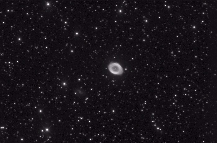
into this:
Here is a final M57 LRGB -- 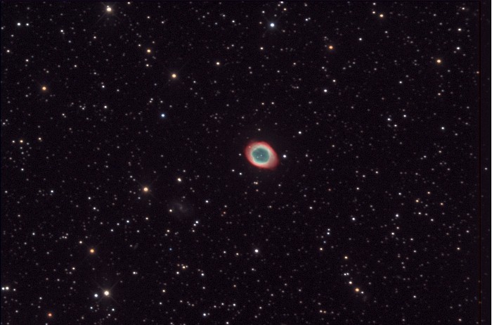
When you have completed your color composite, save it as a TIFF or an uncompressed JPEG so that you can import a no-data-loss color composite file into your favorite post-processing graphics program for any finishing touches.